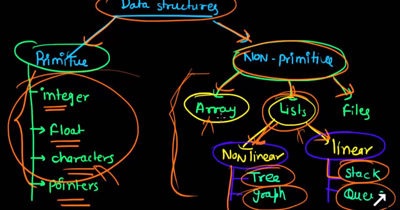
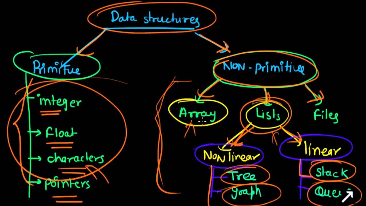
 Different types of Data Structures
The first post of the series briefly defined what a data structure is and its use case. Let me remind you, just in case. Data structures are methods of storing and organizing data in a computer system so that operations can be performed upon them more efficiently. When data is “unstructured,” it does not have a defined data model or is not organized in a manner that is conducive to operations or analysis.
With so much data that we generate every day, you can rest assured that a lot, like a massive load of the data in the world, is unstructured. That’s an opportunity worthy of commercial exploration, let’s structure the data, shall we.
Data structures take the form of different layouts, each of which is efficient for some operations but inefficient for others. The ultimate goal of a programmer is to determine which data structures are suitable for the data on hand so that data can be leveraged to solve problems. Easy enough? Let’s see
1. Arrays
This is the simplest data structure, I believe I can go ahead and make the conclusion that you all know arrays, you have read about them, you have implemented them, probably a dozen times over. Anyway, an array is a collection of items that are stored sequentially. An array contains values or variables — known as “elements” — of the same data type and is of a fixed size, so you cannot change the size of an array. Each item in an array is indexed starting with 0, this is true for pretty much all programming languages.
Because of their simplicity, arrays are commonly used as structures for building other, more complex data structures. They are also used for sorting algorithms. We will get to sorting later, it’s tons of fun I promise.
Program implementation of an Array
/***************************************
// Array Implementation
// Author: Andile Jaden Mbele
***************************************/
#include <iostream>

using namespace std;

int main()
{
    // implement an array of integers
    int array[5] = {1, 2, 3, 4, 5};

    // implement an array of strings as cars
    string cars[5] = {"BMW", "Audi", "Mercedes", "Volvo", "Toyota"};

    // implement an array of strings as rockets
    string rockets[5] = {"Falcon 1", "Falcon 9", "Falcon Heavy", "Falcon Heavy", "Falcon Heavy"};

    // print the first element of the array of rockets
    cout << rockets[0] << endl;
    // print the last element of the array of cars

    cout << cars[4] << endl;
    // print the last element of the array of integers

    cout << array[4] << endl;
    // print all the elements of the array of rockets
    for (int i = 0; i < 5; i++)
    {
        cout << rockets[i] << endl;
    }

    return 0;
}
2. Linked List
I’m not too sure about the commonality of this one, if you have taken any classes on data structures, yes you know this one, if like myself you know Python then you most probably know Lists, not quite Linked Lists though. Linked Lists also seem to be popular in coding technical interviews, I know individuals who were asked to reverse a Linked List on a whiteboard.
A linked list is a sequence of items arranged in a linear order all connected. I like the way you’re thinking, yes you must access data in order, so random access is out of the question with this data structure. Each element in a linked list is called a node, and each node contains a key and a pointer. The pointer directs to the next node, called a next. The sequence starts with a head, which directs you to the first element within the list. The last element of this list is known as, you guessed it — the tail.
There are three types of linked lists, a singly linked list, a doubly-linked list, and a circular linked list. A singly linked list will let you traverse(visit) each item in a forward direction from the head to the tail. Similarly, a doubly-linked list can be traversed both forward and backward. And finally, a circular linked list is one in which the next pointer of the tail points to the head and vice versa, forming a circle hence — circular.
Linked Lists are used in multiple applications including the implementation of stacks and queues which we will get to. Also, they are used in maintaining directories of names.
Program implementation of a Linked List
class Node:
    def __init__(self, data):
        self.data = data
        self.next = None  # make None as the default value for next.


def count_nodes(head):
    # assuming that head != None
    count = 1
    current = head
    while current.next is not None:
        current = current.next
        count += 1
    return count


nodeA = Node(6)
nodeB = Node(3)
nodeC = Node(4)
nodeD = Node(2)
nodeE = Node(1)

nodeA.next = nodeB
nodeB.next = nodeC
nodeC.next = nodeD
nodeD.next = nodeE

print("This linked list's length is: (should print 5)")
print(count_nodes(nodeA))
3. Stacks
A Stack works almost exactly as it sounds. It’s like stacking elements within a tall container. Think of stacks like you would think of a stack of plates waiting to be washed or a stack of cards.
Stacks are known as LIFO (Last In First Out) structures. This means the element placed last can be accessed first. You can push a new element onto the top of the stack, or you can pop, deleting the element inserted last which is at the top of the stack. The peek operation in a stack returns the topmost element in the stack.
Stacks are commonly used for parsing and evaluating mathematical expressions and to implement function calls in recursion programming.
Program implementation of a Stack
/*
Implement a stack with the following methods:   push, pop, peek, and isEmpty.

@Author: Andile Jaden Mbele
*/

public class Stack {

    //let's first store the stack elements in an array
    private int[] stack;
    //the top of the stack is the index of the last element in the array
    private int top;
    //total capacity of the stack
    private int capacity;


    //constructor
    public Stack(int capacity) {
        this.capacity = capacity;
        this.stack = new int[capacity];
        this.top = -1;
    }

    //push an element to the stack
    public void push(int element) {
        if (top == capacity - 1) {
            System.out.println("Stack is full");
            return;
        }
        stack[++top] = element;
    }

    //pop an element from the stack
    public int pop() {
        if (top == -1) {
            System.out.println("Stack is empty");
            return -1;
        }
        return stack[top--];
    }

    //peek the top element of the stack
    public int peek() {
        if (top == -1) {
            System.out.println("Stack is empty");
            return -1;
        }
        return stack[top];
    }

    //check if the stack is empty
    public boolean isEmpty() {
        return top == -1;
    }

    //check if the stack is full
    public boolean isFull() {
        return top == capacity - 1;
    }

    //print the stack
    public void printStack() {
        if (top == -1) {
            System.out.println("Stack is empty");
            return;
        }
        for (int i = top; i >= 0; i--) {
            System.out.print(stack[i] + " ");
        }
        System.out.println();
    }

    //main method
    public static void main(String[] args) {
        Stack stack = new Stack(5);
        stack.push(1);
        stack.push(2);
        stack.push(3);
        stack.push(4);
        stack.push(5);
        stack.printStack();
        System.out.println(stack.pop());
        System.out.println(stack.pop());
        System.out.println(stack.pop());
        System.out.println(stack.pop());
        System.out.println(stack.pop());
        System.out.println(stack.pop());
    }
}
The implementation of the stack code above covers all the stack operations, push, pop, peek, and boolean isEmpty. To push a new element to the stack we have to figure out if the stack is not already full. If the stack is already full, the program returns a message letting the user know no new element additions would be possible. And, if the stack is not empty then the new element is added to the top of the stack.
A similar logic applies as well when we’re popping or deleting an element, we first need to check if the stack has anything inside and if there is we can proceed to delete, else we return a message that lets the user know the stack is empty.
4. Queues
A queue functions similarly to a Stack, but instead of being a LIFO structure, it is a FIFO (First In First Out) structure. The easiest way to think about a Queue is to think of a line of people waiting to be served, at a bank for example. The person at the beginning of the line will be served first, while the person at the end will be served last.
You can enqueue an element in this structure, which means inserting the element to the end of the queue. You can also dequeue an element, which means deleting an element from the beginning of the Queue. Queues are often used to manage threads in multithreading, and they are used to implement priority queuing systems. No surprise there.
Program implementation of a Queue
public class Queue {
    //total capacity of the queue
    private int capacity;
    //front and rear of the queue
    private int front, rear;
    //array to store the elements of the queue
    private int[] queue;

    //constructor
    public Queue(int capacity) {
        this.capacity = capacity;
        this.front = this.rear = -1;
        this.queue = new int[capacity];
    }

    //enqueue an element to the queue
    public void enqueue(int element) {
        if (rear == capacity - 1) {
            System.out.println("Queue is full");
            return;
        }
        queue[++rear] = element;
    }

    //dequeue an element from the queue
    public int dequeue() {
        if (front == rear) {
            System.out.println("Queue is empty");
            return -1;
        }
        return queue[++front];
    }

    //peek the front element of the queue
    public int peek() {
        if (front == rear) {
            System.out.println("Queue is empty");
            return -1;
        }
        return queue[front];
    }

    //check if the queue is empty
    public boolean isEmpty() {
        return front == rear;
    }

    //check if the queue is full
    public boolean isFull() {
        return rear == capacity - 1;
    }

    //print the queue

    public void printQueue() {
        if (front == rear) {
            System.out.println("Queue is empty");
            return;
        }
        for (int i = front + 1; i <= rear; i++) {
            System.out.print(queue[i] + " ");
        }
        System.out.println();
    }
}
5. Hash Tables
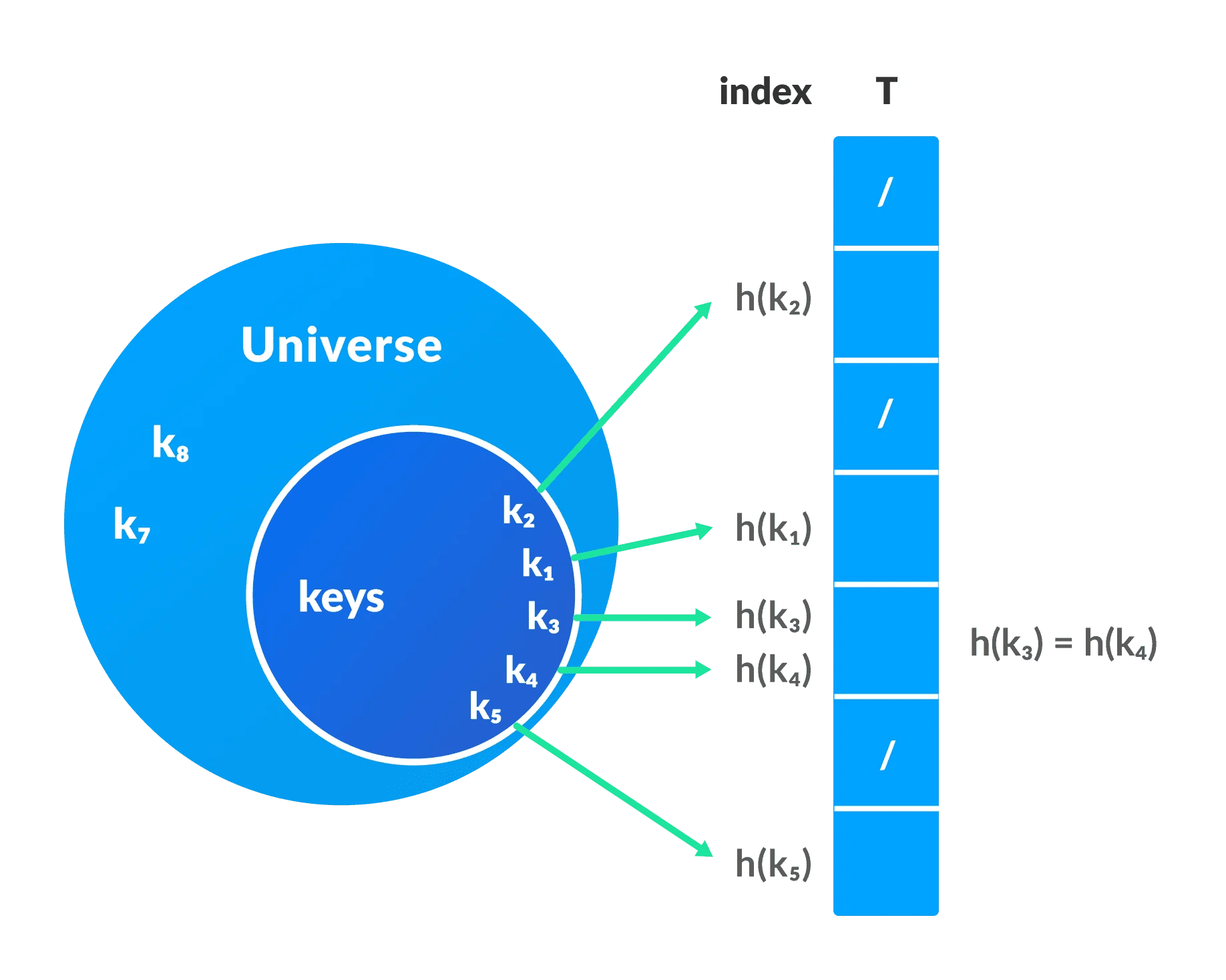
A hash table structure associates each value with a key and then stores them. This makes it easy to look up values efficiently using a key. It’s an efficient way to insert and search for data regardless of its size, as it makes it easy to identify a specific object from a group of similar objects.
For example, if you go to college, you may be assigned a unique student ID number. This ID number is a key that can be used to retrieve information about you and your student record. This process is called hashing. A hash table uses what’s known as a “hash function” to map a data set of any size to one of a fixed size — the hash table. The values that a hash function returns are known as “hash values.”
Hash table Representation
You may be wondering if hash tables are in fact dictionaries… Not quite. A hash table is a loosely typed (non-generic) collection, this means it stores key-value pairs of any data type. A dictionary, on the other hand, is a generic collection meaning it can store key-value pairs of specific data types.
Hash tables are commonly used to create database indexes, create associative arrays and create a “set.” They are also common in cryptographic applications. Program implementation of a hash table
Python program to demonstrate working of a HashTable
# -*- coding: utf-8 -*-
"""
Created on Mon Apr 18 12:10:20 2022

@author: Andile Jaden Mbele
"""
hash_table = [[], ] * 10

def check_prime(n):
    if n == 1 or n == 0:
        return 0

    for i in range(2, n//2):
        if n % i == 0:
            return 0

    return 1

def get_prime(n):
    if n % 2 == 0:
        n += 1
    while not check_prime(n):
        n += 2

    return n

def hash_func(key):
    capacity = get_prime(10)
    return key % capacity

def insert_data(key, data):
    index = hash_func(key)
    hash_table[index] = [key, data]

def remove_data(key):
    index = hash_func(key)
    hash_table[index] = 0

insert_data(123, "Falcon 9")
insert_data(432, "Falcon Heavy")
insert_data(213, "Starship")
#insert_data(276, "Delta IV")
insert_data(654, "Soyuz MS-15")


print("Original Hash Table")
print(hash_table)

remove_data(123)

print("Modified Hash Table")
print(hash_table)
6. Trees
A tree is a structure similar to a linked list because each item is linked. But in a tree items are linked in a hierarchal fashion, just like you might see in a visual representation of someone’s family tree. There are various types of trees, each suited to different applications.
Perhaps one of the most popular, a binary search tree (BST) stores data in sorted order with every node in the binary comprised of the following attributes:
- Key (the value saved in the node)
- Left (pointer to the left child node)
- Right (pointer to the right child node)
- P (pointer to the parent node)
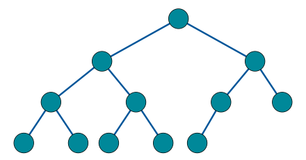
Binary tree
Binary search trees are used in many different types of search applications. Other types of trees are used in wireless networking and to create expression solvers.
Binary Tree Representation looks like this
struct Node
{
  int data;
  struct Node *left;
  struct Node *right;
};
Program implementation of a Binary Tree
# Binary Tree
class Node:
    def __init__(self, key):
        self.left = None
        self.right = None
        self.val = key

    # Traverse preorder
    def traversePreOrder(self):
        print(self.val, end=' ')
        if self.left:
            self.left.traversePreOrder()
        if self.right:
            self.right.traversePreOrder()

    # Traverse in order
    def traverseInOrder(self):
        if self.left:
            self.left.traverseInOrder()
        print(self.val, end=' ')
        if self.right:
            self.right.traverseInOrder()

    # Traverse postorder
    def traversePostOrder(self):
        if self.left:
            self.left.traversePostOrder()
        if self.right:
            self.right.traversePostOrder()
        print(self.val, end=' ')

root = Node(1)

root.left = Node(2)
root.right = Node(3)

root.left.left = Node(4)

print("Pre Order Traversal: ", end=" ")
root.traversePreOrder()

print("\nIn Order Traversal: ", end=' ')
root.traverseInOrder()

print("\nPost Order Traversal", end=' ')
root.traversePostOrder()
7. Heaps
Similarly, a heap is a type of binary tree in which the parent nodes are compared to their children. This allows the values within the nodes to be arranged accordingly. Heaps can be represented as trees, but they can also be represented as binary arrays. They are sometimes called complete binary trees.
There are two types of heaps, min-heap and max heap. In a min-heap, the parent’s key is less than or equal to the keys of its children. In a max heap, the parent’s key is greater than or equal to the keys of its children.
Heaps are often used in algorithms to create priority queues and to find the smallest or largest value in an array and Dijkstra’s Shortest Path Algorithm. In a later post, you will see how I will use the max heap on the Kth Permutation Problem.
Program implementation of a Heap
# -*- coding: utf-8 -*-
"""
Created on Mon Apr 18 13:08:06 2022

@author: Andile Jaden Mbele
"""

def heapify(L, n, i):
    largest = i
    l = 2 * i + 1
    r = 2 * i + 2

    if l < n and L[i] < L[l]:
        largest = l

    if r < n and L[largest] < L[r]:
        largest = r

    if largest != i:
        L[i],L[largest] = L[largest],L[i]
        heapify(L, n, largest)

def insert(array, new_num):
    size = len(array)
    if size == 0:
        array.append(new_num)
    else:
        array.append(new_num);
        for i in range((size//2)-1, -1, -1):
            heapify(array, size, i)

def delete_node(array, num):
    size = len(array)
    i = 0
    for i in range(0, size):
        if num == array[i]:
            break

    array[i], array[size-1] = array[size-1], array[i]

    array.remove(num)

    for i in range((len(array)//2)-1, -1, -1):
        heapify(array, len(array), i)

arr = []

insert(arr, 3)
insert(arr, 4)
insert(arr, 9)
insert(arr, 5)
insert(arr, 2)

print ("Max-Heap array: " + str(arr))

delete_node(arr, 4)
print("After deleting an element: " + str(arr))
8. Graphs
A graph is an abstract, non-linear data structure that is made of a finite set of nodes that are connected by edges. The nodes may be referred to as “vertices” and contain values, whereas the edges are simply lines or arcs that connect two nodes in the graph.
Graphs are often used to represent networks, such as circuit networks or even paths in a city. They are great for solving real-world problems, but they can also be used as representations of digital networks.
For example, on Facebook, each user could be represented with a node (or vertex). Each vertex could then contain information about that user, and each edge could represent its connection with another user.


In the graph above, this is what we can deduce…
V = {0, 1, 2, 3}
E = {(0,1), (0,2), (0,3), (1,2)}
G = {V, E}
Terminology used in graph data structure
Adjacency: A vertex is said to be adjacent to another vertex if there is an edge connecting them. For example vertices 2 and 3 are not adjacent because there is no edge between them.
Path: A sequence of edges that allows traversal from vertex A to vertex B is called a path. 0–1, 1–2 and 0–2 are paths from vertex 0 to vertex 2.
Directed Graph: A graph in which an edge (u,v) doesn’t necessarily mean that there is an edge (v,u) as well. The edges in such a graph are represented by arrows to show the direction of the edge.
Graph Representation
Graphs are represented in two ways i.e. Adjacency Matrix and Adjacency List.
1. Adjacency Matrix
An adjacency matrix is a two Dimensional array of v*v vertices. Each row and column represents a vertex.
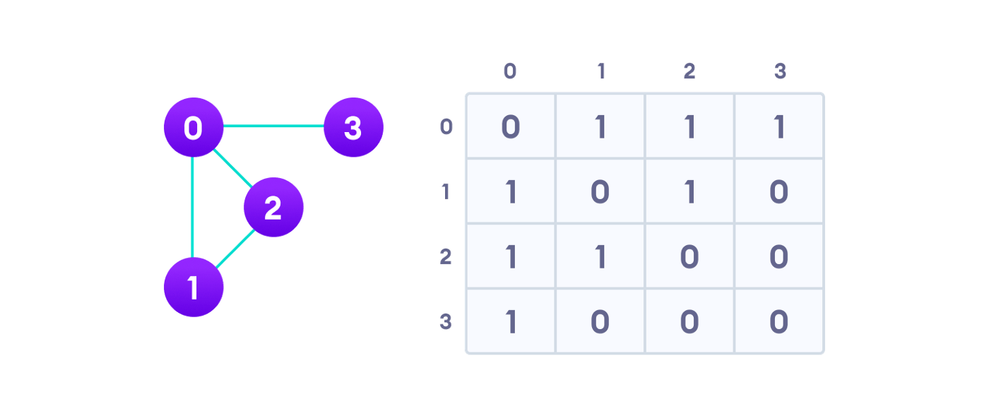
The graph we have is an undirected one, we can tell that by the absence of pointing arrows. We represent relationships between the vertices by using binary (0 and 1). 0 indicates that there’s no relationship between the two vertices we’re looking at and 1represents the presence of a relationship. Since this is an undirected graph, edge (0,2) will be marked true and the same applies for edge (2,0) as well.
2. Adjacency List
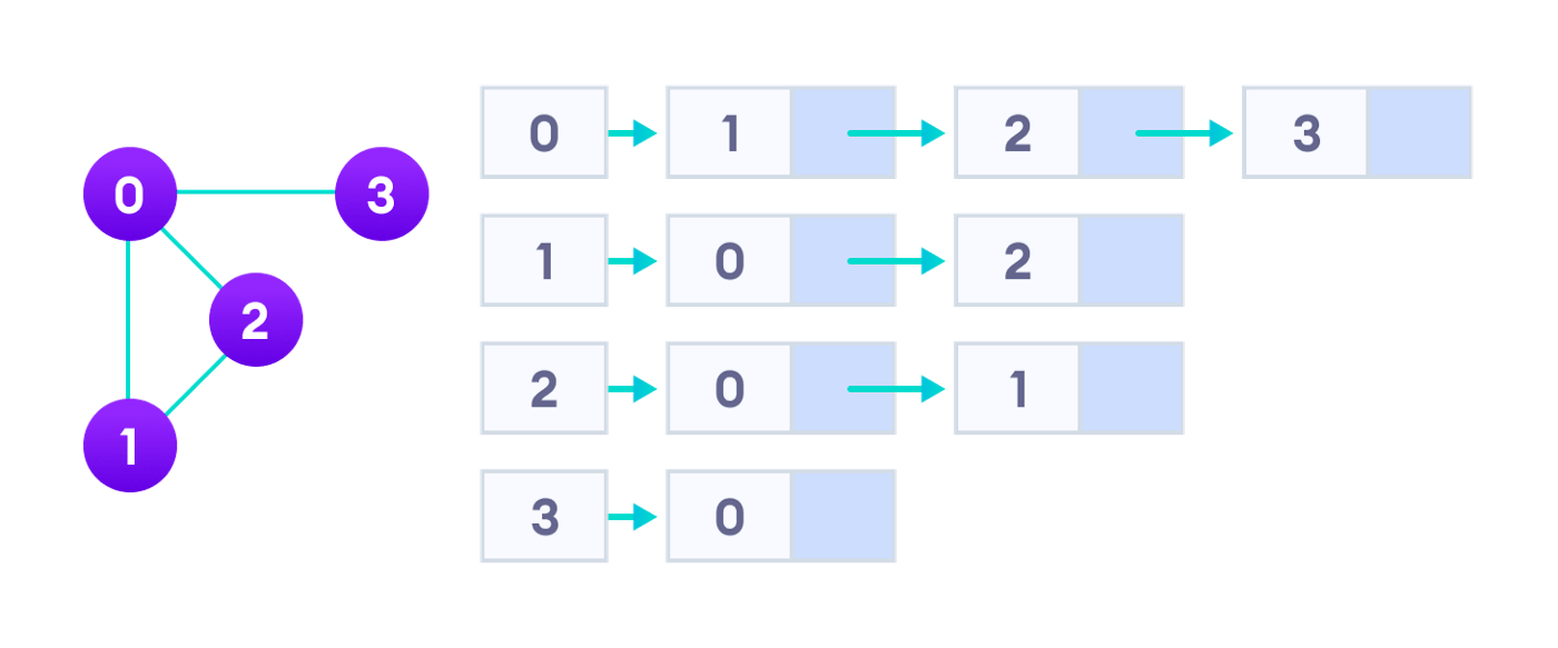
An adjacency list represents a graph as an array of a singly linked list. An array index represents a vertex and each connected element represents the other vertices that form an edge with the vertex.
Graphs help define the flow of computation of software programs. Google Maps implements graphs in building transportation systems. In a Google Map, the intersection of two or more roads will represent the node while the road connecting two nodes represents an edge.
There are two very popular and quite important algorithms in use today that use the Graph data structure in their implementation. The two algorithms are Depth First Search (DFS) and Breadth-First Search (BFS). Underneath you will see the implementation of the Depth First Search Algorithm.
# -*- coding: utf-8 -*-
"""
Created on Mon Apr 18 14:04:47 2022

@author: Andile Jaden Mbele
"""

#Depth First Search Algorithm

def depth_first_search(graph, start, visited=None):
    if visited is None:
        visited = set()
    visited.add(start)

    print(start)

    for next in graph[start] - visited:
        depth_first_search(graph, next, visited)
    return visited

graph = {'0': set(['1', '2']),
         '1': set(['0', '3', '4']),
         '2': set(['0']),
         '3': set(['1']),
         '4': set(['2', '3'])}


depth_first_search(graph, '3')
# Depth First Search in Python
Thank you for reading up to this point, I did not intend to make this a very long article but you know how it is sometimes, stuff just keeps coming. Much appreciated. I hope you learned something new today.
Happy Hacking!
